Summaries#
Scale-free and oscillatory spectral measures of sleep stages in humans (Schneider et. al. 2022)#
Motivation-
The paper intends to investigate the scale-free and oscillatory characteristics of sleep stages in humans. It explores the spectral measures associated with different sleep stages and aims to understand the neurophysiological basis of it.
Source data-
The Budapest-Munich database of sleep records comprises whole night PSG Data collected from 251 healthy subjects, their age ranging from 4 to 69 years. Subjects were divided into 4 age groups - children (4–10 years, N =31), teenagers (10–20 years, N = 36), young adults (20–40 years, N = 150), and middle-aged adults (40–69 years, N= 34) (Bódizs et al., 2021a)
Methodology-
[A]. PSD Calculation :
EEG signals were divided using 4s sliding window while employing 50% overlap(2s step).
Windows containing artifacts were rejected.
Each window was Hanning tapered.
FFT was applied to these tapered windows using mix-radix procedure, a variant of FFT algorithm suitable for windows of arbitrary length.
Welch’s method was applied to obtain the average power-spectral density.
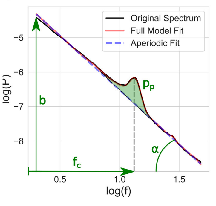
[B]. Model fitting : The authors have used the “fitting oscillations and one over f” (FOOOF) method to extract parameters from the power spectra.
A first approximation of the aperiodic component is calculated using a power-law equation, which is then subtracted from the original spectrum to obtain a flattened version of the spectrum.
The flattened spectrum is analyzed to identify and fit Gaussian functions that represent the periodic components (spectral peaks). These Gaussians are iteratively fitted and subtracted from the flattened spectrum.
The total periodic component is removed from the original spectrum, resulting in a peak-removed spectrum.
The aperiodic component is fitted again to the peak-removed spectrum.
The final result is a combination of the fitted aperiodic and periodic components.
Schneider et. al. 2022
[C]. Parameter Extraction : Several parameters were selected for analysis from the fitted spectra, which are : spectral slope, center frequency, power of the spectral peak with the highest power. The analysis included an alternative spectral intercept, which is determined as the intersection of the fitted power-law at the frequency of the largest oscillatory peak.
The extracted spectral parameters were analyzed using ‘repeated measures ANOVA with sigma restricted parametrization’. The analysis included these categorical factors- Sex(M/F), Age group(4), Sleep stages(W, N1, N2, N3, REM), Brain region, Laterality.
Results-
Spectral slope:
Average slope value reported highest in the wake state
Average slope value decreased through NREM sleep stages
Steeper slopes reported in younger subjects
Steeper slopes in anterior recording regions
Spectral slope value depicted increase with ageof subjects.

Schneider et. al. 2022
Intercept:
Alternative intercept measure was adopted, calculated at frequency of largest peak
Significant sleep stage main effect [F(4,836) = 35.73, p < 0.00001, η2p = 0.15] indicating increased intercepts in the slow-wave sleep stages
Age main effect [F(3,209) = 26.37, η2p = 0.27], with the intercept being higher in children.
Stage-region interaction was observed [F(16,3344) = 9.18, p < 0.00001, η2p = 0.04]. The increase in intercepts was more pronounced in the frontopolar and frontal regions.

Schneider et. al. 2022
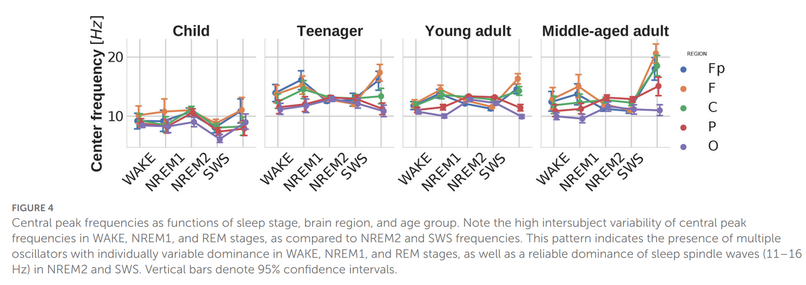
Peak Central Frequency:
The central frequency of the peak with the highest power was increased in the frontal and frontopolar regions.
A significant main effect of region [F(4,824) = 58.138, p < 0.00001, η2p = 0.22], indicating differences in central frequencies across brain regions.
Dominant peak frequencies converged to characteristic sleep spindle frequency in NREM2 stage, most consistent in teenagers.
Increased theta activity observed in NREM1 due to changes in aperiodic component, but the dominant peaks resulted from alpha oscillations (Riedner et al., 2016; Cakan et al., 2022).
Schneider et. al. 2022
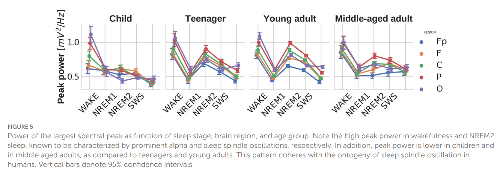
Peak power:
Significant main effects of sleep stage [F(4,824) = 88.765, p < 0.00001, η^2p = 0.301]and brain region [F(4,824) = 97.645, p < 0.00001, η^2p =0.321] were found for the power of the strongest spectral peak
Peak power exhibits prominence in NREM2 stage in younger adults and declines with age.
Schneider et. al. 2022
Adjusted Spectral slope:
To obtain subject-independent measure, by subtracting wake stage slope from other stages of individual subjects.
Exhibits stronger sleep stage main effect and stage-region interaction.

Schneider et. al. 2022
Discussions-
The spectral slope proved to be a strong indicator of sleep stages. The EEG spectral slopes suggest that wakefulness exhibits antipersistent Brownian motion, while sleep is characterized by persistent Brownian motion. State-specific values were adjusted by normalizing them against wakefulness-derived values, leading to even more reliable findings than using absolute values. Sleep stages exhibited a fine-tuned decrease in exponent relative to wakefulness, from -0.2 to -1 in NREM1 and SWS stages.
The findings not only confirm the effects of sleep stages on EEG spectral slopes but also support the age and region dependency previously reported in studies (Voytek et al., 2015; Bódizs et al., 2021b; Pathania et al., 2022). Steeper spectra was a notable feature in younger subjects and in more anterior regions of brain. The most significant age-related flattening of EEG spectral slopes was observed in SWS, and antero-posterior differences in spectral steepness were particularly prominent in this stage. Additionally, the findings suggested that the alternative and adaptive spectral intercept is independent of the slope, providing non-redundant sleep stage effects when analyzing these intercepts.
Central peak frequencies in EEG reflected neural oscillatory patterns specific to different sleep stages. Alpha activity (8-12 Hz) observed in resting wakefulness, sleep spindles (11-16 Hz) in NREM sleep stages including SWS, and theta (4-8 Hz) or beta (16-30 Hz) in REM sleep. Stable wake state alpha frequency observed in children. NREM2 and SWS stages exhibit prominent sleep spindle frequencies with antero-posterior differences, while NREM1 and REM sleep show beta oscillations with anterior predominance.
The study found that high peak power values are characteristic of wakefulness and NREM2 sleep, lowest in NREM1 and REM, and intermediate in SWS.These findings align with known patterns of alpha and sleep spindle oscillations. Age-related changes in peak power indicate an initial increase in sleep spindle frequencies during teenage/young adult years, followed by a decrease in middle-aged adults.
However, the study has limitations, such as missing age ranges, differences in sleep scoring rules, and assumptions about Gaussian spectral peaks.Despite these limitations, the results suggest that spectral parameters can serve as objective measures for characterizing sleep states, potentially enabling automated sleep evaluation.
Compute the average bandpower of an EEG signal (Raphael Vallet)#
The tutorial demonstrates how to compute the average band power of an EEG signal in a specific frequency range using Python. The tutorial talks about Welch’s periodogram method and the multitaper spectral estimation method of EEG signal processing.
The flow of the code is as follows:
Import necessary libraries: NumPy, SciPy, SciPy. Integrate, matplotlib, seaborn
Load EEG Data
Define parameter: sample rate, time
Plot the signal
Compute power spectral density using Welch’s method
Compute average delta band power using Simpson’s rule
Compute relative band power
The tutorial uses the following concepts and methodologies:
FFT: FFT is a mathematical tool which decomposes a signal into its constituent frequencies. It represents a signal in the frequency domain.
Power Spectral Density: PSD is given by the magnitude squared of Fourier transform. It provides information about the strength of the constituent frequencies in the signal.
Welch’s Periodogram: Welch’s periodogram estimates the PSD of a signal. Welch’s method improves the accuracy of the classic periodogram in EEG signal processing. It does so by dividing the data into shorter segments, computing separate periodograms for each segment, and averaging them. This accounts for the time-varying nature of EEG signals and reduces bias and variance, resulting in a more reliable spectral analysis. However, this method comes at the cost of low frequency resolution.
Frequency resolution: Fres = 1/t = 1/30 = 0.033 (t= time duration of signal)
Optimal window duration = 2/ lowest freq. of interest = 2/0.5 = 4s (for delta freq)
Note:
The only thing that increases frequency resolution is time. Changes in sampling frequency do not increase the frequency resolution but only the frequency coverage.
The maximum value of the x-axis of a Welch’s Periodogram is always half the sampling frequency of the original signal.
Simpson’s Rule: It’s an integration method used to approximate the area under the curve. The area can be decomposed into several parabola and then summed up. Here, it has been used for integrating the psd values within the range of a frequency band to estimate average band power.
Multitaper Method: This method was developed to overcome the limitations of classical spectral estimation techniques. It combines the advantages of classical and Welch’s periodograms to provide better spectral estimation with high frequency resolution and low variance. The method involves filtering the signal with optimal bandpass filters known as Slepian sequences, calculating a periodogram for each filtered data, and averaging the results. However, this method is computationally intensive and hence much slower than Welch’s method.
FOOF Documentation#
FOOOF is a tool for parameterizing neural power spectra. It models the power spectrum as a combination of an aperiodic component (1/f slope) and periodic components (peaks over the 1/f slope).
The benefit of using FOOOF is that it characterizes the peaks in the power spectrum in terms of their center frequency, power, and bandwidth without the need to predefine specific bands of interest for the aperiodic component. It also provides a measure of the aperiodic component itself.
FOOOF is written in python and is object-oriented.There is a Matlab wrapper that allows you to use FOOOF from Matlab.
FOOOF works on frequency representations of power spectra in linear space. FOOFGroup can be used to fit a group of power spectra
To fit a single power spectra -
# Import the FOOOF object
from fooof import FOOOF

# Initialize FOOOF object
fm = FOOOF()

# Define frequency range across which to model the spectrum
freq_range = [x, y]

# Model the power spectrum with FOOOF, and print out a report
fm.report(freqs, spectrum, freq_range)
FOOOF has settings for the algorithm -
# Initialize a FOOOF model object with defined settings
fm = FOOOF(peak_width_limits=[z, w], max_n_peaks=a, min_peak_height=g,
peak_threshold=b , aperiodic_mode='fixed')
To fit a group of Spectra -
# Import FOOOFGroup
from fooof import FOOOFGroup

# Initialize FOOOFGroup object
fg = FOOOFGroup(peak_width_limits=[z, w], max_n_peaks=a)

# Fit spectra and save results
fg.fit(freqs, spectra)
fg.save_report()
fg.save(file_name='fooof_group_results', save_results=True)